An Introduction To SQL Using Hockey Stats

6 years ago

While hockey statistics work is often done with languages like R or Python that require a reasonable amount of programming knowledge to take advantage of, there are simpler tools that can be used to accomplish many tasks. I still use spreadsheets for a significant chunk of the stats work I do. However, managing data in spreadsheets can become cumbersome past a certain point, and it’s not the greatest way to organize large data sets. Thankfully, there’s a programming language that’s designed specifically to aid in data management, and it’s not too difficult to start learning even if you don’t have any kind of background in writing code. That language is SQL, and this post is an introduction to how to use it, with all the examples constructed using hockey data.

Before I get into any actual SQL, I want to outline what this post is and what it isn’t. The goal of this article is to provide a starting point for people who have little or even no knowledge of SQL. That means that if you do have a background in coding or already know some SQL, you might find this a little basic. I might follow this post up with another one digging into some more complex examples, but for the moment my goal is to help beginners get started and provide a basic framework for understanding how SQL works.

This article has been written with the idea that you can get your own SQL instance set up and try out everything I describe as you read along. The best way to learn how a programming language works is to start writing with it, so everything here is laid out so you can recreate it yourself. I’ll provide the code necessary to accomplish all the tasks we’ll go through, and there will be links to download data sets for you to import and play around with.

Like with any programming language, there are often a number of ways to accomplish the same things using SQL. I don’t claim that the approach outlined here is the “best” way to perform any given task; my goal is to explain things in a way that makes it easy to learn how SQL works.

FIRST STEPS

Before you can write any code or load any data, you’ll need a database program to work with. There are a number of popular options, but for this article I’ve chosen to go with PostgreSQL (commonly shortened to “Postgres”). I picked it for a few reasons. The primary one is that it’s completely free and open source, so you’re getting a fully-featured database without needing to spend any money. Postgres is available on Windows, Mac, and Linux, so no matter what operating system you’re using to read this article, you can run Postgres on it. It’s also a system I’ve used professionally, so I’m more familiar with its particular quirks. Unfortunately SQL is not a completely standardised language, so while code that works in Postgres will usually work in other database programs like Microsoft SQL Server, that’s not always the case.

The PostgreSQL web site is located here if you want to know more about the program, and the installer can be downloaded at this link. Select version 9.6.5, and then select your operating system. If you’re on Windows and you’re not sure whether you have a 32 or 64 bit operating system, open the Start menu, right click on “Computer” and select “Properties” – the screen that loads contains that information. Install Postgres using all the default settings. At the end of the installation it may ask if you want to install Stack Builder; say no.

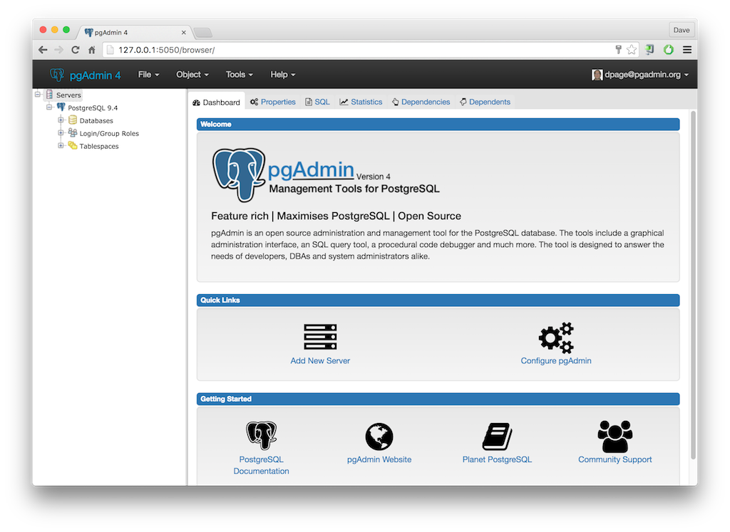
Once Postgres is installed, the interface you use to manage your databases is in a program installed alongside PostgreSQL called “pgAdmin”. Run pgAdmin, and you should see an interface that looks something like this:

The next thing we want to do is create a database for all of the statistics we want to keep track of. Right-click on Databases and select Create > Database. In the Database field, enter the name “SQL Tutorial” and then click Save. You can ignore all the other options for now.

Great, now you’ve got a database! But you can’t actually do anything with it until we create some tables and populate them with data.

CREATING YOUR FIRST TABLES

Expand the SQL Tutorial table tree by clicking the + symbol beside it. You’ll see a series of other options that won’t make a lot of sense to you at the moment, but right now there’s only one we need to pay attention to. It’s the one at the bottom called Schemas. Expand Schemas and then expand public. You can create any number of schemas, but for this article we’re going to stick with the defaults.

Under Schemas > public you should see an entry called Tables – that’s where most of your data is actually going to go. Many of the tasks in Postgres can be simplified by using the built-in wizards, but since the goal of this tutorial is to help you learn some SQL, we’re going to do most things with code instead. Even if you use the wizards later on, it’s good to understand how things actually work under the hood.

So let’s create our first table. This one’s going to be pretty small just so you can get a sense of how everything works. The first table is going to hold some career statistics for the Hockey Hall of Fame’s 2017 class. Right-click on Tables and select Query tool. This is the main interface used for writing SQL code. In the query tool, type this code, which will create the table:

CREATE TABLE public."Hall of Fame"
 (
 "Player" character varying,
 "Games Played" integer,
 "Goals" integer,
 "Assists" integer,
 "Points" integer
 )

Once the text is all there, press F5, which is the key that runs the code you’ve typed (you can also click on the Execute button near the top of the screen, which does the same thing).

What does that code actually do? Thankfully SQL commands are often pretty close to plain English, so you can probably figure a lot out just by looking at the code. Let’s break it down:

CREATE TABLE is the command to create a new table, as you’d expect
public.”Hall of Fame” is the name we’re giving the table and the schema to place it under; in Postgres the names of things like tables and columns get placed in double quotes, while text strings are placed in single quotes (I’ll get into more detail on this shortly)
the rest is the list of columns that we want to add, which goes inside brackets
when creating a column the name you want to give the column goes inside double quotes, followed by the type of data that you want to store
there are a wide variety of data types available in Postgres, but we’re going to stick with some basic ones here – character varying is just a way of saying you want to store text, while integer stores whole numbers (no decimals); if you want to store decimal places you would generally use the data type real, but integers take up less memory and are quicker in calculations so it’s better to use integers if you know you’ll never need decimals

A table without any data in it isn’t very useful, so now we need to actually insert the players and their career stats into the table. Once we start working with bigger data sets later on we’ll use an import wizard, but since we’re starting small let’s do it all in code for now. Delete all the SQL you wrote earlier in the query editor and then type this:

INSERT INTO public."Hall of Fame"
("Player", "Games Played", "Goals", "Assists", "Points")
VALUES ('Teemu Selanne', 1451, 684, 773, 1457),
('Dave Andreychuk', 1639, 640, 698, 1338),
('Paul Kariya', 989, 402, 587, 989),
('Mark Recchi', 1652, 577, 956, 1533)

There are a few things to point out here about data formatting, because like most code, SQL will not work correctly if you don’t use the right formatting:

as described above, table and column names go in double quotes; if you put them in single quotes you’ll get an error
text strings go in single quotes, like the player names above; if you put them in double quotes you’ll get an error
numbers can just be written as normal, with no need for quotation marks

If you haven’t done so already, press F5 to run the query. Now we’ve actually got a table populated with some data to work with.

USING THE DATA

The first thing you probably want to do is take a look at the table you’ve created. To load data and look at it we use a command called SELECT, and the most simple form of the SELECT command just grabs everything in a table. Delete any SQL you have visible in the query editor and then run this:

SELECT *
FROM "Hall of Fame"

SELECT * just means ‘select all of the columns’ and FROM tells Postgres which table has the data you want to see. If everything has gone correctly up until this point, you should see a table that looks like this:

This looks a lot like any spreadsheet program you might have used in the past, but one key difference with a SQL table is that you can’t do anything directly to the data in this view. For example, you can’t click in a column and modify it. If you want to actually change any of the data or the way that it displays, you have to do that with code.

So let’s reorganize our results a bit. We’re going to re-order the table so that the players are displayed from most career points to fewest. The new code looks very similar to the code we ran above, but now we’re adding a new line to the end, like this:

SELECT *
FROM "Hall of Fame"
ORDER BY "Points" desc

You can order your results in either ascending (asc) or descending (desc) order (if you don’t put asc or desc it will use ascending order by default). This does not actually change the way the data is stored, it’s just modifying the way it’s displayed on screen. You can confirm that for yourself by deleting the ORDER BY line and running the query again, which will put the display back to the original format.

This is a small table so we don’t mind looking at the whole thing at once, but normally you want to limit how much data you’re viewing at any given time. We do that with the WHERE clause. If we only wanted to look at the players in this list with at least 1000 career points, we would add an additional line to our SQL code, like this:

SELECT *
FROM "Hall of Fame"
WHERE "Points" >= 1000
ORDER BY "Points" desc

You may have noticed that I’ve added the WHERE line before the ORDER BY line. That’s because SQL generally requires that your commands be written in a specific order. If you swap the WHERE and ORDER BY lines, it will produce a syntax error. You’ll get a better handle on how the ordering works as you write more SQL.

In a moment we’re going to move on to some larger data sets and more complicated data selection, but it might be a good idea to try playing around with the commands you’ve learned so far to practice writing your own code without being able to rely on the example code I’ve provided. For example, can you figure out how to write SQL to narrow the list down to the two players who’ve scored over 500 goals AND 700 assists?

WORKING WITH BIGGER DATA SETS

The previous section was just an introduction so you could get a handle on how SQL looks and the basic structure of tables. You might be thinking that this is kind of boring, and you want to know how to use Postgres with some real data. I don’t want to get too complicated in this article, since the goal is to introduce you to SQL and how it works, but let’s pull in some of the kind of data that you might actually want to store in a database.

Hockey Reference very conveniently lets you export any of its tables to the CSV format, which is a format we can easily import into a SQL database. I’ve grabbed all of the standard statistics Hockey Reference tracks for every skater who played in the NHL in either the 2015-16 or 2016-17 seasons and put them in CSVs that you can use. Please download both seasons:

If you’re not familiar with CSV files, you can try opening one of these in a text editor like Notepad.

These files have a lot of columns in them, far more than you probably want to type out one-by-one. Postgres does have a wizard to create tables more quickly. You can see what it looks like by right-clicking on Tables, then select Create > Table. On the Columns tab you can add as many columns as you want and give them names, data types, and so forth. However, to keep things moving along I’m going to give you some SQL to enter in the query editor that will give you everything you need. Run this code:

CREATE TABLE public."SkaterStats1516"
(
 "Name" character varying,
 "Games Played" integer,
 "Team" character varying(3),
 "League" character varying(3),
 "Position" character varying(2),
 "Season" character varying(7),
 "Age" integer,
 "Goals" integer,
 "Assists" integer,
 "Points" integer,
 "+/-" integer,
 "PIM" integer,
 "EV Goals" integer,
 "PP Goals" integer,
 "SH Goals" integer,
 "GW Goals" integer,
 "Shots" integer,
 "S%" real,
 "TOI" integer,
 "Goals Per Game" real,
 "Assists Per Game" real,
 "Points Per Game" real,
 "Shots Per Game" real,
 "OPS" real,
 "DPS" real,
 "Point Shares" real
)

There are a couple of new details here that you haven’t seen in any of the previous SQL statements:

the data type real is now being used for some columns; that’s because they need decimal places, which integer columns won’t hold
some of the text fields now have a number in brackets after them – this indicates the maximum length of the field, which we know in some cases (like the league name) will never go over a certain number of characters; the primary reason to do this is for data quality – if you tried to import a row where the “Position” field was 12 characters, it would throw an error and you would know something was wrong with your data (be prepared to spend a lot of time doing data cleanup and normalization if you ever really get into working with SQL)

And let’s create the table for the 2016-17 season as well. Since the two tables will hold identical columns, just change the name from “SkaterStats1516” to “SkaterStats1617” in the SQL code above, then run the query again.

Now we need to put some data into the tables, which is contained in the CSV files I linked to above. Because we’re putting in so much data now it would be a waste of time to enter it all by hand, so we’ll use the import wizard that’s built into Postgres. Right-click on the table “SkaterStats1516” and select Import/Export. Follow these steps to finish the data import:

Click the blue Export button near the top of the screen to change it to Import.
Click the … next to the Filename field and select the file 1516_stats_allskaters.csv which you downloaded earlier.
Under the Header option click the blue No to change it to Yes (you will get an error if you don’t do this because the first line in the CSV contains field names).
Click on the Delimiter drop-down and select the comma (which is the most commonly used separator between fields in CSV files, but there are exceptions).
Switch to the Columns tab. Since we want to import data for every column in the table, leave this as it is and click on OK at the bottom of the screen.

If everything has been done correctly up to that point, you should see a success message very quickly.

Now follow the same procedure to import the 1617 stats into the 1617 table.

You probably want to see what the data looks like, so using what you learned earlier, perform a SELECT on one of these tables.

It’s neat to be able to see all of the data at once, but not very useful, so let’s look at a new way of limiting our results, which is to only SELECT specific columns. Try this:

SELECT "Name", "Shots", "Goals", "S%"
FROM "SkaterStats1516"

The resulting table is a lot more readable. If we want to only look at stats related to goal scoring, it’s easier to pull only those columns rather than having to scroll back and forth through the table. You may have also noticed that I changed the field order here. That’s something else you can do in a SELECT clause, but remember that the underlying data is not modified at all; the column order is only changed in the current view.

So far we haven’t really done anything that you couldn’t do in a spreadsheet, although you can do a lot of these things more quickly in SQL once you become familiar with how to write queries. One of the things that SQL is good at is combining information from multiple tables. Most SQL databases are “relational”, which means that the different tables link together, usually using a system of IDs known as “primary keys”. So you might have one table with a list of player biographical information, a series of tables with the stats for each season, and so forth, and rather than listing the player’s info in every single table, you’d just list their ID, and you could pull the other information by linking the results (I’ll demonstrate this concept, called a JOIN, in a moment).

I’ve avoided having you set up primary keys for the data in these exercises to simplify the process. As it happens, there are no duplicate player names in the data that I’ve provided, so names can operate essentially as unique IDs, but in a real database this would be a bad idea (for example, there may be two players named “Sebastian Aho” in the NHL next season).

We’ve currently got two databases full of player statistics, and by now hopefully you have an idea of how to pull information for players from one season. But what if you wanted to combine the information from both tables? This is done through a JOIN statement, which finds rows that match between two tables and combines them into one new row. There are a few new concepts to introduce here, so let’s start with performing one simple addition: games played. We’ll add up GP for every player in the two tables and output it beside their name.

SELECT s1."Name", 
 s1."Games Played" + s2."Games Played" as "GP"
FROM "SkaterStats1516" s1
FULL JOIN "SkaterStats1617" s2 on s2."Name" = s1."Name"

Let’s go through the new ideas in that code:

this query uses something called aliases and it uses two different forms of them – one for table names and one for column names
it would get annoying to have to type out “SkaterStats1516” every time we want to refer to that table, so we can assign it a temporary name (an alias) to use just in this query; I’ve shortened the first table to s1 (for “season one”) and the other to s2
you can also give an alias to a table name (or in this case, the result of some arithmetic between two tables), by saying SELECT [column name] as “[alias]”
you can perform arithmetic in a SELECT statement, like the simple addition done above

I’ve also introduced the concept of a JOIN, which is one of the central ideas in relational databases. JOINs are the most complicated idea I’m introducing in this article, so let’s break down all of the new elements here:

there are several types of JOINs; in this post I’m sticking to just one kind, the FULL JOIN
when you perform a JOIN you list the JOIN type, then the table you want to connect to your base table; it’s kind of like another FROM clause
next you list the criteria you want to use to determine if there is a match; in this case, I’m saying ‘If there are rows in table 1 and table 2 with the same “Name”, combine those into one row”
a FULL JOIN will combine all the rows that match between the two tables; it will also return results for all player names that are found in one season, but not the other; the other types of JOIN would omit at least some of those rows (this is a more advanced concept for another day)

Here’s a colour-coded image that might make this more clear:

red = JOIN type
blue = table we want to combine with our base table
green = criteria to use to check if the data matches

If you’ve taken some time to look at the data from that last query, you may have noticed that we’ve actually made a mistake here. Some of the rows have null values in either the “Name” or “GP” field. That’s because for the rows that have no match in the other table, Postgres is assigning the value null to the result. You can’t add an integer to a null value, so what we need to do is tell Postgres to replace any null values with zero.

We have a similar problem with the names. Since we’re only pulling names from the 2015-16 table, any player who is only in the 2016-17 data is not having their name pulled. We can fix both these problems using a command called COALESCE. (Coalescing will make the SQL look a bit ugly and it’s kind of a pain to type out, but it’s how we get around the null values and it’s simpler than other methods we might use. Sometimes SQL code just requires a lot of grunt work.)

To use COALESCE we pass a series of values into the SELECT clause. When the query is executed, it goes through each value and stops when it finds the first one that’s valid. So, for example, if we type the following:

COALESCE (s1."Name", s2."Name")

It will return the value in the “Name” column from table s1 if it exists. If it doesn’t exist it will look at the “Name” field in table 2 instead.

This is what our previous query should look like after updating it to account for possible null values:

SELECT COALESCE(s1."Name", s2."Name"),
 COALESCE(s1."Games Played",0) + COALESCE(s2."Games Played",0) as "GP"
FROM "SkaterStats1516" s1
FULL JOIN "SkaterStats1617" s2 on s2."Name" = s1."Name"

Now we’ve got a bit of a toolkit of things we can do with SQL, so let’s put it all together and run a query that’s a little bit closer to the kind of thing you might actually want to look up. Maybe we want to find the cut-off for the scoring total of a top pair defenceman over the past two seasons, a player in the top 60 in scoring among defencemen. We could write a query that looks like this:

SELECT COALESCE(s1."Name", s2."Name"),
 COALESCE(s1."Games Played",0) + COALESCE(s2."Games Played",0) as "GP",
 COALESCE(s1."Goals",0) + COALESCE(s2."Goals",0) as "G",
 COALESCE(s1."Assists",0) + COALESCE(s2."Assists",0) as "A",
 COALESCE(s1."Points",0) + COALESCE(s2."Points",0) as "PTS"
FROM "SkaterStats1516" s1 
FULL JOIN "SkaterStats1617" s2 on s2."Name" = s1."Name"
WHERE s1."Position" = 'D' or s2."Position" = 'D'
ORDER BY "PTS" desc
LIMIT 60

There’s one new idea in there, which is the LIMIT clause. As you have probably guessed, it limits the resulting table to the number of results you specify.

CLOSING THOUGHTS

That’s the end of the concepts I want to cover in this post. I admit that most of the exercises in this article covered things you could easily do on Hockey Reference without needing to know any coding, but it’s important to learn the basics before moving on to more advanced concepts. I hope that at the very least now you have some ideas about things that you could explore using SQL, and you should have a bit of knowledge that will let you mess around with the data I’ve provided and try writing some queries of your own. You’ll probably run into a few error messages, but that’s fine – everyone runs into errors, and figuring out how to fix them is a good way to learn some of the details of how a programming language works.

If you’ve finished reading this article and tried out the examples, please let me know whether you found it helpful. If you have any questions about things I didn’t cover or things I did cover that weren’t clear, feel free to get in touch. If there’s enough interest, I’d like to write a second article that introduces a few more advanced concepts (like setting up keys between tables to create a properly relational database) and digs into some more concrete examples of things you can do with SQL to explore hockey data. If there’s anything in particular you think would be interesting to learn about, let me know, and I’ll see how much I can fit into another piece later this month.

If you want to provide some feedback you can post a comment below, e-mail me at draglikepull at yahoo dot com, or reach out to me on Twitter @draglikepull (but it might be hard to answer coding questions in 140 characters). If you’ve stuck with this through the 4000+ words, thanks for reading, and I hope you’ve found it useful.

Uncategorized